
The US has one of the highest COVID-19 per capita infection rates in the world. Many factors have contributed to this unfortunate honor, including the Trump administration's bungled response to the pandemic, the Trump administration's bungled response to the pandemic, and also the Trump administration's bungled response to the pandemic. I'm here reminded of Richard Clarke's testimony at the 9/11 commission which he opened with an apology: Your government failed you. Those entrusted with protecting you failed you. I failed you. I suspect we'll get no such apology from The Donald.
The good news -- if we can call it that -- is because of Trump's stunning malfeasance, the humble SIR model is a better description of the COVID pandemic than it otherwise would be. Intervention complicates disease dynamics, adding terms to the equations and expanding the search space of parameters we need to fit. In the absence of a public health response, we're left with only three classifications -- susceptible (S), infected (I), and removed (R) -- and two parameters -- the transmission (β) and recovery (γ) rates -- which describe both our model and our fate.
Additionally, the longer COVID drags on the more data we have to test. Of course, none of the numbers can be trusted as long as Trump lackeys have opportunity to spike the CDC spreadsheets. Videre quam esse, and all that. However, that, too, can be good thing, for it allows us to check if model parameters match what healthcare workers are reporting from the trenches. Any discrepancy indicates malarkey may be afoot, kinda like how Neptune was discovered by analyzing the discrepancies of Uranus.
So, let's fire up Matlab and fit a COVID model. We're all sequestered at home this happy holiday, so what else is there to do?
Our point of departure is the SIR epidemiology model, which we have met in other LabKitty missives. In contrast to our previous discrete time COVID model, this time we go full differential equation monty, because why not. It provides an excuse to review solving differential equations in Matlab, which is a good skill to have what with numerical solutions often being the only solutions we can get on the damn things. (One might wonder how such a rarely-cooperative tool became the gold standard in technical fields. I have waxed philosophical in re this topic elsewhere. But I digress).
Long story short: Matlab requires you to create a function file that defines the ODE of interest which you then feed to one of its solvers along with initial conditions and a time interval. Mathworks provides quite a few solvers. There's ode45, ode113, ode15s, ode23s, ode23t, ode23tb, ode15i, as well as odeset, odeplot, odephas2, odephas3, and odeprint. The variants generally trade runtime for stability, with the Matlab docs having much to say about solving "stiff" equations. My experience is is they either all work or none of them do. If you ever find yourself cycling though the list late one night because your first choice produced garbage, you are probably up to no good.
Footnote: If you'd like to go the free alternative route, Octave is pretty good in the ODE department and even offers solvers with a Matlab-compatible interface.
The details are more easily shown than described, so I will just provide example code. Here's one way to describe the SIR epidemiology model as a Matlab ODE function:
The function returns [S(t),I(t),R(t)] in the variable dydt. NB: The solver might pass in a vector of t values because reasons, so your code can't assume t is a scalar. (Here the issue is moot because t doesn't explicitly appear in the equations, but FYI.)
You can pass parameters to an ODE function by listing them in the function definition after the required parameters t and y. I pass in the transmission and recovery rates using b and g, respectively, because they were the closest letters to β and γ that live on my keyboard.
Put the above code in an mfile SIR.m (Matlab will suggest the name when you save the file).
To use our ODE function, we pass it to one of the solvers. I'm using ode23:
The generic syntax goes:
The argument initial_conditions is a vector of initial conditions -- one for each entry in y. For the SIR model this is [S(0) I(0) R(0)], provided here by the variables S0, I0, and R0. The argument timevec can be just a two-element vector [t_start t_final]. If you pass in a full vector as I did here, then the y values returned will be evaluated at those particular values (in the two-element version, y is returned at whatever values the solver picks based on convergence criteria).
Finally, the argument odefunc is a handle to your ode function. The Matlab syntax for this is a bit wonky. If we had not elected to pass parameters b and g to the function (we could instead define them as globals) the syntax simplifies:
However, we do, ergo the ugly syntax shown earlier. Them's the breaks.
The function returns the solution in matrix y, evaluated at the times returned in t. This makes for easy plotting.
Here's my code all in one place:
We set values of b, g, and the initial conditions, call ode23, and plot the results. Later we'll stick this in a loop to do parameter fitting.
Here's some example output:
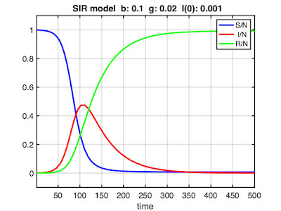
Note the y-axis is scaled [0 1] because we're using a normalized model (i.e., we don't work with counts of S, I, and R, but rather the proportions S/N, I/N, and R/N, where N is the total population size). This is not strictly required, but it allows us to compare epidemics in different-sized populations. (Also, the only published COVID models I could find were normalized, so I had to normalize to compare parameter values.) The x-axis scaling would be in whatever time units (days, months, etc.) γ is expressed.
Footnote: Always check whether a model is normalized when comparing model parameters.
Footnote: In a normalized model, we sometimes use the term fraction instead of proportion (e.g., the "infected fraction"). Also, I might slip and write "number of," even though it's technically incorrect.
Presumably, if we picked appropriate values of b and g, our model would model the current US COVID-19 pandemic.
How do we do that?
The approach used by people who know what they're doing* is to take field data and derive parameters theoretically. After all, we know their epidemiology interpretation: β defines the rate of contagion and γ is the reciprocal of the mean infectious period.
However, I'll obtain model parameters via fitting. After all, there's only two parameters which makes searching the parameter space straightforward. It doesn't even require a very sophisticated algorithm. Simply bracket a range of feasible values, generate a bunch of solutions, test each one against the available data, and pick the parameter combination that minimizes, say, the squared error.
But before getting into fitting, it's useful to see how the parameters affect model dynamics. For that, we take a brief detour into a gallery of SIR models.
A Gallery of SIR Models
We really have three not two parameters to fit. There's β and γ and also the initial conditions -- that is, the number of susceptible, infected, and removed at time zero. If we're lucky the parameters won't interact much, making it easier to search the parameter space for optimal values.
To familiarize you with parameter effects, I made a few plots. Each plot shows the model output for a combination of β, γ, and I(0), with two held constant and the third varied over the range shown in the plot title. Susceptible, infected, and removed are plotted in blue, red, and green, respectively, with color saturation increasing with increasing value of the varied parameter (so all three curves would be black for the first parameter combination and pure R,G,B for the last). The parameter values are not special, but rather were chosen to illustrate typical model behaviors.
The first example is shown below:
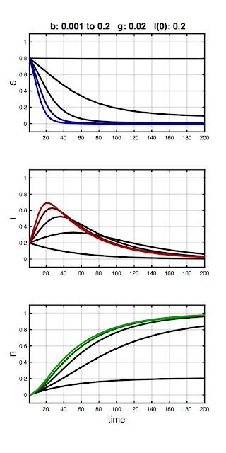
Here, γ and I(0) are fixed, while β increases from 0.001 to 0.2. As you can see, the initial combination of parameters result in no epidemic (black traces). A peak then emerges in the infected fraction as β increases. We can understand this in epidemiology terms: The overall infection rate is proportional to the infection rate per contact (β) times the total time infected (1/γ). As such, if the the recovery rate (equivalently: infectious period) is held constant, an outbreak won't occur until β exceeds some threshold. Otherwise, the number of infecteds simply declines monotonically from I(0). This break-even point is called the basic reproduction ratio (R0). More on R0 in a bit.
Stare at the plot until corresponding red curves, blue curves, and green curves make sense. Helpful tip: the values of the blue, red, and green curves at any time must add to 1. Members of the population are simply moving between S, I, and R compartments.
Footnote: Forcing a peak in the number of infecteds by increasing β for a fixed value of γ is something we will exploit later in parameter fitting.
In the next plot, I hold β constant and vary γ :
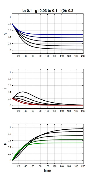
This series demonstrates a complementary effect to the first, with the initial parameter combination resulting in an epidemic (black traces) which is then quashed as γ increases. Again, we can understand this in terms of dynamics: contagion can be contained for a constant infection rate (β) if the window of opportunity to spread the disease is sufficiently shortened.
In the final plot, I hold β and γ constant and vary the number of initial infecteds:
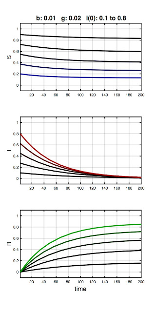
Here I(0) is ranges from 0.1 to 0.8. Note the infected fraction monotonically returns to zero, and does so over approximately the same time course, regardless of initial value. That is, the size of the initial infected population does not qualitatively alter the disease dynamics. In fact, the qualitative dynamics of the SIR model are wholly determined by the relative magnitudes of β and γ, quantified in the basic reproduction ratio: R0 = β / γ.
Think of R0 as the number of people each infected person infects. We must have R0 > 1 for an "epidemic" to occur, the definition being an increase in the number (or fraction) of infecteds over the initial value (and not simply that infecteds are present in the population). Conversely, if R0 < 1 then the infected fraction monotonically decreases, regardless of the initial number. We can observe this at work in the plots. For example, in the first plot no epidemic occurred until β exceeded 0.02 (which it did in the second step). And in the last plot, R0 = β / γ = 0.01 / 0.02 = 0.5, which tells us an epidemic cannot occur, and in this series of models none did.
Footnote: If using unnormalized (i.e., count) data, then R0 is calculated as βN / γ. You will get the same value of R0 regardless because β will be different.
Footnote: Don't confuse R0 with R0, the initial size of the removed class in the code listing. Eventually, variable names start to look alike.
Now that we have a feel for how model parameters affect model dynamics, we're ready to fit our model to data. To do so, we require data to fit it to. And for that, we head to the Internet.
COVID-19 Data
The Wikipedia page on the COVID pandemic has a sidebar listing infections and deaths by day starting in January 2020. They cite the source of the data as "official reports from state health care professionals" whatever that means. Presumably that means the CDC, but I couldn't make heads or tails out of the data hosted on the official CDC website. The rows there are "whichever state last called in" and the columns are a mishmash of "tot cases" and "conf cases" and "prob cases" and what-all else. For the love of Cats, I just need a plot of infections v. time.
As such, we're going with the Wikipedia numbers. I cut and pasted these into Matlab and plotted. Here's total US infections from the end of January 2020 to when I'm working on this (mid-December 2020):
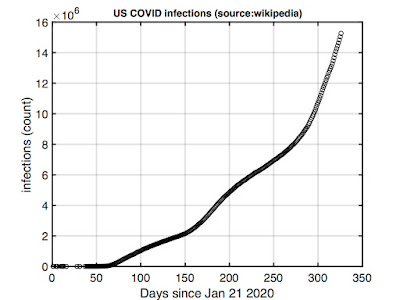
Note this is count data -- we'll divide by the total population size (328 million) to normalize before fitting.
The curve suggest we're still on the upswing of the pandemic. It's not the pure exponential growth an SIR model would predict, but it's not too far off. The deviations may reflect early mitigation efforts (recall the "flatten the curve" call of last summer) which appear to now be losing to an overall upward trend.
We can exploit this feature to simplify parameter fitting. From our previous exploration, we know that, for a fixed value of γ, increasing β will eventually cause a peak to emerge in the number of infections. But the observed data is not peaked. This suggests a search strategy: If we can bracket γ (more on that in a moment), we can increment β for each value of γ starting at zero and stopping once a peak emerges in the predicted response. We can then move to the next value of γ. We test all possible pairs, then pick the best one.
Which leaves the problem of bracketing the recovery rate. Here we turn to observations on the CDC website:
There's one final fitting issue. You might think we begin with I(0) = 1 -- a literal patient zero that got the ball rolling, so to speak. The problem is the SIR is a "mass action" model and mass action models break down at small numbers. As such, throwing out the first few months of data when I(t) and R(t) were small should result in more meaningful parameters (because the assumptions of the model are then better met).
For example, here's the best fit I could obtain if we use all of the Wikipedia data (starting at January 21 2020 with one infected):
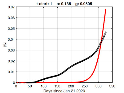
We're obviously being penalized by what the SIR model can do. It isn't designed to suppress growth for two months, so forcing it to do so results in a poor fit.
We can obtain more meaningful parameters by omitting some of the initial data -- there's not much sense in fitting the early epidemic where a mass action model breaks down anyway. Here's fitting results after discarding the first 50 points (note change in the x-axis):
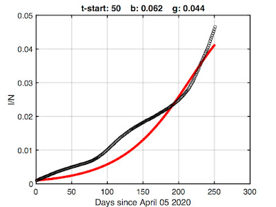
There's still some undershoot (if I allowed the model to match the early growth, its exponential growth overwhelms the latter) but this is probably the best we're going to get while retaining as much data as we can. So let's go with it.
As shown in the title, the resulting best-fit model parameters are β = 0.062 and γ = 0.044. We could rerun the fitting at a finer resolution using these as starting values, but extra precision is silly given the simplicity of the SIR model.
Footnote: The 50th entry in the Wikipedia data is for April 05, 2020. There were 333593 confirmed infections and 9534 deaths.
So, how do these model parameters compare with published values?
A value of γ = 0.044 corresponds to an infectious period of 1/0.044 or about 23 days. That's midrange in the CDC values assuming an infectious presymptomatic period. Interestingly, because we derived this value from population data (rather than, say, from a blood test), it suggests the presymptomatic infectious period meaningfully affects disease spread. That's not some stunning revelation; it's why reasonable voices have been urging social distancing and mask wearing.
To evaluate β it's easier to instead compare the R0 predicted by our model. This quantity is more often cited in the literature, probably because it has direct implications for epidemic dynamics.
Wikipedia lists an R0 range of 3.28 to 5.7 for COVID-19. However, it's important to ask when and where when scrutinizing published values (also how, as there's different ways to calculate R0, from regression to Markov Chain Monte Carlo). If you dig into the bibliography on that Wikipedia page, you'll find the article cited analyzes only the early outbreak in Wuhan (and they actually report a range of 3.8 to 8.9).
A better source for comparison is an August 20 report in Clinical Epidemiology and Global Health which lists R0 values between 1.00011 and 2.7936 depending on location ("location" = India, the Syrian Arab Republic, the United States, Yemen, China, France, Nigeria, or Russia). The value they give for the US is 1.6135 (Table 2), this based on a modified SIR model which includes a deceased category.
Using our fitted values of β and γ, our model predicts R0 = β / γ = 1.41. I'd say that's not too shabby for amateur epidemiology.
Here's the fitting code:
This more-or-less implements what is described above, looping over a bracket of γ values while incrementing β, testing the squared error in the model fit, and stopping when a peak emerges in the infected fraction. Other details are noted in the comments. I omitted the code that returns the COVID data -- it's simply the Wikipedia numbers returned in three vectors (time, infections, deaths) with the tops trimmed off by the value passed to the function. (NB: the Wikipedia data skips some days in January and February.)
Model Predictions
Now that we have a working model, we can take it out for a spin. What you probably want to see is how the pandemic will play out, This is extrapolation, which is always a dicey proposition (see next section), but prediction is a big raison d'être of modeling. It's one way epidemiology is used to inform public policy (or used to be, back when grownups were in charge).
I ran an SIR model using the values of β and γ we fitted above we and increased t_final until the number of infected returned to zero. Here's the result:
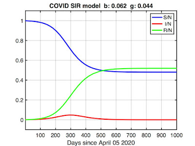
The model predicts the epidemic will peak around day 300 (about March 2021, given our starting time of April 05, 2020) before finally disappearing in late summer (day 500 or so). The infected fraction (red curve) may look inconsequential, but remember the vertical axis is scaled so that 1.0 = the total population (~328 million). The peak represents about 15 million in real numbers.
The more troubling curves here are the susceptible (blue) and removed (green) fractions. The model predicts about half the country will get infected by the time the pandemic subsides (R(t_final) ≅ 0.5). This may seem dubious, but it's not worse than worst-case scenarios some epidemiologists have described. Tragically, it's also insufficient for herd immunity (which requires closer to 90% immunity), leaving open the possibility of future outbreaks.
But the more dire implication is the removed fraction (R), which in the SIR model comprises both recovered and deceased. Multiplying R(t_final) by N, our model predicts about 170 million will become infected. Assuming the current observed COVID fatality rate of 1-2% continues to hold -- higher can be expected if healthcare resources get overwhelmed -- that translates to approximately three million dead.
To put that number into perspective, three million was about the total number of annual deaths in the US prior to COVID. From all causes. It's more people than the population of any city in the US except Los Angeles or New York. It's more than the entire population of a third of the states. It's about 6x the number of Americans killed in WW II, 60x the number killed in the Korean or Vietnam war, and about 1000x number of Americans who died in the 9/11 attacks.
All-in-all, a rather unnerving projection.
What are we to make of it?
Postscript: The Ghosts of Christmas Future
We will know in time if our model is correct. More data will arrive, and these can be compared with the predictions. If the model and the data don't agree -- and fingers crossed they do not -- we might reasonably conclude the model is wrong. Either the parameterization is wrong or the COVID pandemic violates one or more critical assumptions of the SIR model.
However, there's an alternative, more nuanced interpretation. As Caswell reminds us:
The situation our data describes was a rudderless America in the grips of COVID-19. The White House was offering no coherent policy, being either unable, or unwilling, or just plain disinterested in managing the crisis. States were left to fend for themselves, fighting a federal government actively subverting their efforts, broadcasting mixed messages in daily briefings, hoarding critical PPE supplies, and encouraging its lunatic fringe to reject distancing and mask mandates to a degree that approached insurrection.
Our model suggests the consequence of those "present conditions" is three million dead.
The most salient development in the COVID-19 pandemic isn't the arrival of a vaccine, it's the results of the November election. A vaccine isn't useful until it is distributed, and there's every reason to believe the Trump administration would have bungled distribution just as it has bungled all aspects of pandemic management. Indeed, it already has. Delayed shipments. Lost shipments. Withheld shipments. Crony prioritism. It's safe to assume vaccination will flounder at least until January 20th, when the Biden administration takes over and we once again have a functioning government. In the meantime, COVID will continue to burn through the country. It's entirely possible three million dead might not be far off the actual final tally.
In the end, this will be Trump's legacy: a mountain of corpses -- every one of them somebody's son or daughter -- because he had no interest in doing the job. That's why you don't elect a person like Donald Trump to high office, or any office.
Go stand in the ashes of three million dead Americans and ask the ghosts if Hillary's emails matter.
The good news -- if we can call it that -- is because of Trump's stunning malfeasance, the humble SIR model is a better description of the COVID pandemic than it otherwise would be. Intervention complicates disease dynamics, adding terms to the equations and expanding the search space of parameters we need to fit. In the absence of a public health response, we're left with only three classifications -- susceptible (S), infected (I), and removed (R) -- and two parameters -- the transmission (β) and recovery (γ) rates -- which describe both our model and our fate.
Additionally, the longer COVID drags on the more data we have to test. Of course, none of the numbers can be trusted as long as Trump lackeys have opportunity to spike the CDC spreadsheets. Videre quam esse, and all that. However, that, too, can be good thing, for it allows us to check if model parameters match what healthcare workers are reporting from the trenches. Any discrepancy indicates malarkey may be afoot, kinda like how Neptune was discovered by analyzing the discrepancies of Uranus.
So, let's fire up Matlab and fit a COVID model. We're all sequestered at home this happy holiday, so what else is there to do?
Our point of departure is the SIR epidemiology model, which we have met in other LabKitty missives. In contrast to our previous discrete time COVID model, this time we go full differential equation monty, because why not. It provides an excuse to review solving differential equations in Matlab, which is a good skill to have what with numerical solutions often being the only solutions we can get on the damn things. (One might wonder how such a rarely-cooperative tool became the gold standard in technical fields. I have waxed philosophical in re this topic elsewhere. But I digress).
Long story short: Matlab requires you to create a function file that defines the ODE of interest which you then feed to one of its solvers along with initial conditions and a time interval. Mathworks provides quite a few solvers. There's ode45, ode113, ode15s, ode23s, ode23t, ode23tb, ode15i, as well as odeset, odeplot, odephas2, odephas3, and odeprint. The variants generally trade runtime for stability, with the Matlab docs having much to say about solving "stiff" equations. My experience is is they either all work or none of them do. If you ever find yourself cycling though the list late one night because your first choice produced garbage, you are probably up to no good.
Footnote: If you'd like to go the free alternative route, Octave is pretty good in the ODE department and even offers solvers with a Matlab-compatible interface.
The details are more easily shown than described, so I will just provide example code. Here's one way to describe the SIR epidemiology model as a Matlab ODE function:
function dydt = SIR(t,y,b,g)
%
% ODE function for the SIR model:
%
% dS/dt = -bSI
% dI/dt = bSI - gI
% dR/dt = gI
%
% b is the transmission rate (beta)
% g is the recovery rate (gamma)
%
dydt = [ -b*y(1)*y(2); b*y(1)*y(2)-g*y(2); g*y(2) ];
end
%
% ODE function for the SIR model:
%
% dS/dt = -bSI
% dI/dt = bSI - gI
% dR/dt = gI
%
% b is the transmission rate (beta)
% g is the recovery rate (gamma)
%
dydt = [ -b*y(1)*y(2); b*y(1)*y(2)-g*y(2); g*y(2) ];
end
The function returns [S(t),I(t),R(t)] in the variable dydt. NB: The solver might pass in a vector of t values because reasons, so your code can't assume t is a scalar. (Here the issue is moot because t doesn't explicitly appear in the equations, but FYI.)
You can pass parameters to an ODE function by listing them in the function definition after the required parameters t and y. I pass in the transmission and recovery rates using b and g, respectively, because they were the closest letters to β and γ that live on my keyboard.
Put the above code in an mfile SIR.m (Matlab will suggest the name when you save the file).
To use our ODE function, we pass it to one of the solvers. I'm using ode23:
[t,y] = ode23(@(t,y) SIR(t,y,b,g), [0:40], [S0 I0 R0]);
The generic syntax goes:
[t,y] = ode23(odefunc, timevec, initial_conditions)
The argument initial_conditions is a vector of initial conditions -- one for each entry in y. For the SIR model this is [S(0) I(0) R(0)], provided here by the variables S0, I0, and R0. The argument timevec can be just a two-element vector [t_start t_final]. If you pass in a full vector as I did here, then the y values returned will be evaluated at those particular values (in the two-element version, y is returned at whatever values the solver picks based on convergence criteria).
Finally, the argument odefunc is a handle to your ode function. The Matlab syntax for this is a bit wonky. If we had not elected to pass parameters b and g to the function (we could instead define them as globals) the syntax simplifies:
[t,y] = ode23(@SIR, [0:40], [S0 I0 R0]);
However, we do, ergo the ugly syntax shown earlier. Them's the breaks.
The function returns the solution in matrix y, evaluated at the times returned in t. This makes for easy plotting.
Here's my code all in one place:
% SIR main code
b = 0.1;
g = 0.02;
t_final = 500;
I0 = 0.001;
R0 = 0.0001;
S0 = 1 - I0 - R0;
[t,y] = ode23(@(t,y) SIR(t,y,b,g),[1 t_final],[S0 I0 R0]);
plot(t,y(:,1),'b',...
t,y(:,2),'r',...
t,y(:,3),'g','LineWidth',3)
bs = [ 'b: ' num2str(b,3)];
gs = [ ' g: ' num2str(g,3)];
is = [ ' I(0): ' num2str(I0,2)];
title(['SIR model ' bs gs is]);
xlabel('time');
legend('S/N',' I/N','R/N');
axis([1 max(t) -0.1 1.1]);
set(gca,'FontSize',16,'LineWidth',2);
grid on;
We set values of b, g, and the initial conditions, call ode23, and plot the results. Later we'll stick this in a loop to do parameter fitting.
Here's some example output:

Note the y-axis is scaled [0 1] because we're using a normalized model (i.e., we don't work with counts of S, I, and R, but rather the proportions S/N, I/N, and R/N, where N is the total population size). This is not strictly required, but it allows us to compare epidemics in different-sized populations. (Also, the only published COVID models I could find were normalized, so I had to normalize to compare parameter values.) The x-axis scaling would be in whatever time units (days, months, etc.) γ is expressed.
Footnote: Always check whether a model is normalized when comparing model parameters.
Footnote: In a normalized model, we sometimes use the term fraction instead of proportion (e.g., the "infected fraction"). Also, I might slip and write "number of," even though it's technically incorrect.
Presumably, if we picked appropriate values of b and g, our model would model the current US COVID-19 pandemic.
How do we do that?
The approach used by people who know what they're doing* is to take field data and derive parameters theoretically. After all, we know their epidemiology interpretation: β defines the rate of contagion and γ is the reciprocal of the mean infectious period.
However, I'll obtain model parameters via fitting. After all, there's only two parameters which makes searching the parameter space straightforward. It doesn't even require a very sophisticated algorithm. Simply bracket a range of feasible values, generate a bunch of solutions, test each one against the available data, and pick the parameter combination that minimizes, say, the squared error.
But before getting into fitting, it's useful to see how the parameters affect model dynamics. For that, we take a brief detour into a gallery of SIR models.
A Gallery of SIR Models
We really have three not two parameters to fit. There's β and γ and also the initial conditions -- that is, the number of susceptible, infected, and removed at time zero. If we're lucky the parameters won't interact much, making it easier to search the parameter space for optimal values.
To familiarize you with parameter effects, I made a few plots. Each plot shows the model output for a combination of β, γ, and I(0), with two held constant and the third varied over the range shown in the plot title. Susceptible, infected, and removed are plotted in blue, red, and green, respectively, with color saturation increasing with increasing value of the varied parameter (so all three curves would be black for the first parameter combination and pure R,G,B for the last). The parameter values are not special, but rather were chosen to illustrate typical model behaviors.
The first example is shown below:

Here, γ and I(0) are fixed, while β increases from 0.001 to 0.2. As you can see, the initial combination of parameters result in no epidemic (black traces). A peak then emerges in the infected fraction as β increases. We can understand this in epidemiology terms: The overall infection rate is proportional to the infection rate per contact (β) times the total time infected (1/γ). As such, if the the recovery rate (equivalently: infectious period) is held constant, an outbreak won't occur until β exceeds some threshold. Otherwise, the number of infecteds simply declines monotonically from I(0). This break-even point is called the basic reproduction ratio (R0). More on R0 in a bit.
Stare at the plot until corresponding red curves, blue curves, and green curves make sense. Helpful tip: the values of the blue, red, and green curves at any time must add to 1. Members of the population are simply moving between S, I, and R compartments.
Footnote: Forcing a peak in the number of infecteds by increasing β for a fixed value of γ is something we will exploit later in parameter fitting.
In the next plot, I hold β constant and vary γ :

This series demonstrates a complementary effect to the first, with the initial parameter combination resulting in an epidemic (black traces) which is then quashed as γ increases. Again, we can understand this in terms of dynamics: contagion can be contained for a constant infection rate (β) if the window of opportunity to spread the disease is sufficiently shortened.
In the final plot, I hold β and γ constant and vary the number of initial infecteds:

Here I(0) is ranges from 0.1 to 0.8. Note the infected fraction monotonically returns to zero, and does so over approximately the same time course, regardless of initial value. That is, the size of the initial infected population does not qualitatively alter the disease dynamics. In fact, the qualitative dynamics of the SIR model are wholly determined by the relative magnitudes of β and γ, quantified in the basic reproduction ratio: R0 = β / γ.
Think of R0 as the number of people each infected person infects. We must have R0 > 1 for an "epidemic" to occur, the definition being an increase in the number (or fraction) of infecteds over the initial value (and not simply that infecteds are present in the population). Conversely, if R0 < 1 then the infected fraction monotonically decreases, regardless of the initial number. We can observe this at work in the plots. For example, in the first plot no epidemic occurred until β exceeded 0.02 (which it did in the second step). And in the last plot, R0 = β / γ = 0.01 / 0.02 = 0.5, which tells us an epidemic cannot occur, and in this series of models none did.
Footnote: If using unnormalized (i.e., count) data, then R0 is calculated as βN / γ. You will get the same value of R0 regardless because β will be different.
Footnote: Don't confuse R0 with R0, the initial size of the removed class in the code listing. Eventually, variable names start to look alike.
Now that we have a feel for how model parameters affect model dynamics, we're ready to fit our model to data. To do so, we require data to fit it to. And for that, we head to the Internet.
COVID-19 Data
The Wikipedia page on the COVID pandemic has a sidebar listing infections and deaths by day starting in January 2020. They cite the source of the data as "official reports from state health care professionals" whatever that means. Presumably that means the CDC, but I couldn't make heads or tails out of the data hosted on the official CDC website. The rows there are "whichever state last called in" and the columns are a mishmash of "tot cases" and "conf cases" and "prob cases" and what-all else. For the love of Cats, I just need a plot of infections v. time.
As such, we're going with the Wikipedia numbers. I cut and pasted these into Matlab and plotted. Here's total US infections from the end of January 2020 to when I'm working on this (mid-December 2020):

Note this is count data -- we'll divide by the total population size (328 million) to normalize before fitting.
The curve suggest we're still on the upswing of the pandemic. It's not the pure exponential growth an SIR model would predict, but it's not too far off. The deviations may reflect early mitigation efforts (recall the "flatten the curve" call of last summer) which appear to now be losing to an overall upward trend.
We can exploit this feature to simplify parameter fitting. From our previous exploration, we know that, for a fixed value of γ, increasing β will eventually cause a peak to emerge in the number of infections. But the observed data is not peaked. This suggests a search strategy: If we can bracket γ (more on that in a moment), we can increment β for each value of γ starting at zero and stopping once a peak emerges in the predicted response. We can then move to the next value of γ. We test all possible pairs, then pick the best one.
Which leaves the problem of bracketing the recovery rate. Here we turn to observations on the CDC website:
Available data indicate that persons with mild to moderate COVID-19 remain infectious no longer than 10 days after symptom onset. Persons with more severe to critical illness or severe immunocompromise likely remain infectious no longer than 20 days after symptom onset.Note this is after symptom onset. The model doesn't care if you're symptomatic; it only cares if you're infectious. A significant COVID pre-symptomatic infectious period has been reported, which is consistent with the pervasive global spread of the disease. The CDC has more info on that:
The incubation period for COVID-19 is thought to extend to 14 days, with a median time of 4-5 days from exposure to symptoms onset. One study reported that 97.5% of people with COVID-19 who have symptoms will do so within 11.5 days.So if my math is correct, γ ranges from about 1/20 to /10 if the asymptomatic are not infectious, and from about 1/34 to 1/15 if they are. This is, of course, predicated on accurate reporting of exposure which is something of an oxymoron. If you don't know you're sick, you don't think about when you got infected. As such, let's just conservatively bracket γ between 1/100 and 1/10.
There's one final fitting issue. You might think we begin with I(0) = 1 -- a literal patient zero that got the ball rolling, so to speak. The problem is the SIR is a "mass action" model and mass action models break down at small numbers. As such, throwing out the first few months of data when I(t) and R(t) were small should result in more meaningful parameters (because the assumptions of the model are then better met).
For example, here's the best fit I could obtain if we use all of the Wikipedia data (starting at January 21 2020 with one infected):

We're obviously being penalized by what the SIR model can do. It isn't designed to suppress growth for two months, so forcing it to do so results in a poor fit.
We can obtain more meaningful parameters by omitting some of the initial data -- there's not much sense in fitting the early epidemic where a mass action model breaks down anyway. Here's fitting results after discarding the first 50 points (note change in the x-axis):

There's still some undershoot (if I allowed the model to match the early growth, its exponential growth overwhelms the latter) but this is probably the best we're going to get while retaining as much data as we can. So let's go with it.
As shown in the title, the resulting best-fit model parameters are β = 0.062 and γ = 0.044. We could rerun the fitting at a finer resolution using these as starting values, but extra precision is silly given the simplicity of the SIR model.
Footnote: The 50th entry in the Wikipedia data is for April 05, 2020. There were 333593 confirmed infections and 9534 deaths.
So, how do these model parameters compare with published values?
A value of γ = 0.044 corresponds to an infectious period of 1/0.044 or about 23 days. That's midrange in the CDC values assuming an infectious presymptomatic period. Interestingly, because we derived this value from population data (rather than, say, from a blood test), it suggests the presymptomatic infectious period meaningfully affects disease spread. That's not some stunning revelation; it's why reasonable voices have been urging social distancing and mask wearing.
To evaluate β it's easier to instead compare the R0 predicted by our model. This quantity is more often cited in the literature, probably because it has direct implications for epidemic dynamics.
Wikipedia lists an R0 range of 3.28 to 5.7 for COVID-19. However, it's important to ask when and where when scrutinizing published values (also how, as there's different ways to calculate R0, from regression to Markov Chain Monte Carlo). If you dig into the bibliography on that Wikipedia page, you'll find the article cited analyzes only the early outbreak in Wuhan (and they actually report a range of 3.8 to 8.9).
A better source for comparison is an August 20 report in Clinical Epidemiology and Global Health which lists R0 values between 1.00011 and 2.7936 depending on location ("location" = India, the Syrian Arab Republic, the United States, Yemen, China, France, Nigeria, or Russia). The value they give for the US is 1.6135 (Table 2), this based on a modified SIR model which includes a deceased category.
Using our fitted values of β and γ, our model predicts R0 = β / γ = 1.41. I'd say that's not too shabby for amateur epidemiology.
Here's the fitting code:
% fit an SIR model to US COVID-19 data
% best fit beta and gamma are put
% in variables bbest and gbest
[ tdata,idata,ddata ] = wikipedia_covid_data(50);
N = 328e06; % US 2020 population 328M
idata = idata / N;
ddata = ddata / N;
S0 = 1 - idata(1);
I0 = idata(1);
R0 = 0; % to 1st approximation
% initialize
binc = 0.001;
gvec = linspace(0.005,0.1,40);
min_diff = Inf;
% search
for g = gvec
b = binc;
while (1)
[t,y] = ode23(@(t,y) SIR(t,y,b,g),tdata,[S0 I0 R0]);
this_diff = idata - y(:,2);
this_diff = dot(this_diff,this_diff);
if (this_diff < min_diff)
min_diff = this_diff;
bbest = b;
gbest = g;
end
% we keep increasing beta until a peak emerges
% then exit the inner loop (because the data
% is not peaked)
%
% the signature is that the max is not the last point
% however, we also have to check that the max isn't
% the first point (i.e. simple exponential decay)
%
% also, lets add a 5 point safety buffer
[~,mindex] = max(y(:,2));
if (mindex+5 < size(y,1) && mindex > 5)
break;
end
b = b + binc;
end
end
This more-or-less implements what is described above, looping over a bracket of γ values while incrementing β, testing the squared error in the model fit, and stopping when a peak emerges in the infected fraction. Other details are noted in the comments. I omitted the code that returns the COVID data -- it's simply the Wikipedia numbers returned in three vectors (time, infections, deaths) with the tops trimmed off by the value passed to the function. (NB: the Wikipedia data skips some days in January and February.)
Model Predictions
Now that we have a working model, we can take it out for a spin. What you probably want to see is how the pandemic will play out, This is extrapolation, which is always a dicey proposition (see next section), but prediction is a big raison d'être of modeling. It's one way epidemiology is used to inform public policy (or used to be, back when grownups were in charge).
I ran an SIR model using the values of β and γ we fitted above we and increased t_final until the number of infected returned to zero. Here's the result:

The model predicts the epidemic will peak around day 300 (about March 2021, given our starting time of April 05, 2020) before finally disappearing in late summer (day 500 or so). The infected fraction (red curve) may look inconsequential, but remember the vertical axis is scaled so that 1.0 = the total population (~328 million). The peak represents about 15 million in real numbers.
The more troubling curves here are the susceptible (blue) and removed (green) fractions. The model predicts about half the country will get infected by the time the pandemic subsides (R(t_final) ≅ 0.5). This may seem dubious, but it's not worse than worst-case scenarios some epidemiologists have described. Tragically, it's also insufficient for herd immunity (which requires closer to 90% immunity), leaving open the possibility of future outbreaks.
But the more dire implication is the removed fraction (R), which in the SIR model comprises both recovered and deceased. Multiplying R(t_final) by N, our model predicts about 170 million will become infected. Assuming the current observed COVID fatality rate of 1-2% continues to hold -- higher can be expected if healthcare resources get overwhelmed -- that translates to approximately three million dead.
To put that number into perspective, three million was about the total number of annual deaths in the US prior to COVID. From all causes. It's more people than the population of any city in the US except Los Angeles or New York. It's more than the entire population of a third of the states. It's about 6x the number of Americans killed in WW II, 60x the number killed in the Korean or Vietnam war, and about 1000x number of Americans who died in the 9/11 attacks.
All-in-all, a rather unnerving projection.
What are we to make of it?
Postscript: The Ghosts of Christmas Future
We will know in time if our model is correct. More data will arrive, and these can be compared with the predictions. If the model and the data don't agree -- and fingers crossed they do not -- we might reasonably conclude the model is wrong. Either the parameterization is wrong or the COVID pandemic violates one or more critical assumptions of the SIR model.
However, there's an alternative, more nuanced interpretation. As Caswell reminds us:
Population projections reveal something about present conditions (more precisely, about the relation between present conditions and the population experiencing them), not about the future behavior of the population. As [British demographer Nathan Keyfitz] has pointed out, one of the most powerful ways to study present conditions is to examine their consequences were they to remain as they are. A speedometer works the same way. A reading of 60 miles per hour predicts that, in one hour, the car will be found 60 miles in a straight line from its present location. As a forecast, this is almost always false. But as a projection, it provides valuable information about the present situation of the automobile. (p. 30)As of this writing, a COVID vaccination program has begun. This should significantly alter the dynamics of the epidemic. As such, the SIR model here does not show the future that will be, but rather the future that would have been had present conditions continued. Present conditions have not continued, but that does not make the predictions any less illuminating.
The situation our data describes was a rudderless America in the grips of COVID-19. The White House was offering no coherent policy, being either unable, or unwilling, or just plain disinterested in managing the crisis. States were left to fend for themselves, fighting a federal government actively subverting their efforts, broadcasting mixed messages in daily briefings, hoarding critical PPE supplies, and encouraging its lunatic fringe to reject distancing and mask mandates to a degree that approached insurrection.
Our model suggests the consequence of those "present conditions" is three million dead.
The most salient development in the COVID-19 pandemic isn't the arrival of a vaccine, it's the results of the November election. A vaccine isn't useful until it is distributed, and there's every reason to believe the Trump administration would have bungled distribution just as it has bungled all aspects of pandemic management. Indeed, it already has. Delayed shipments. Lost shipments. Withheld shipments. Crony prioritism. It's safe to assume vaccination will flounder at least until January 20th, when the Biden administration takes over and we once again have a functioning government. In the meantime, COVID will continue to burn through the country. It's entirely possible three million dead might not be far off the actual final tally.
In the end, this will be Trump's legacy: a mountain of corpses -- every one of them somebody's son or daughter -- because he had no interest in doing the job. That's why you don't elect a person like Donald Trump to high office, or any office.
Go stand in the ashes of three million dead Americans and ask the ghosts if Hillary's emails matter.
* DISCLAIMER: LabKitty is not an epidemiologist. For reliable COVID information, seek out a reputable source such as the COVID dashboard at Johns Hopkins University or the World Health Organization.

No comments:
Post a Comment